Multi-objective Reinforcement Learning

How can we handle a vector of rewards in the context of reinforcement learning?

What is Multi-objective Reinforcement Learning

Reinforcement learning is classically known to optimize a policy that maximizes a (scalar) reward function. However, in many problems, we encounter several objectives or rewards that we care about; sometimes, the objectives are conflicting with one another. For example, in robotic locomotion, we want to maximize forward velocity but also minimize joint torque and impact with the ground. The subfield of reinforcement learning that deals with multiple objectives, i.e., a vector reward function rather than a scalar, is called Multi-objective reinforcement learning (MORL)

In the MORL domain, there are two standard approaches that are usually taken:

1) The \(\textbf{single-objective}\) practice is to use a scalar objective function that is a weighted sum or a function of all the objectives. In this regard, it is sometimes common to order or rank the objectives for choosing the appropriate weights; and also order or rank the solutions obtained. However, it is not only difficult to determine how to weigh the objectives, but also often harder to balance the factors to achieve satisfactory performance along all the objectives. Often, the scalar objective is simply taken to be the sum of the individual objectives.

2) The alternative \(\textbf{Pareto}\) starategy tries to find multiple solutions to the MORL problem that offer trade-offs among the various objectives. In other words, these multiple solutions, also called \(\textbf{Pareto solutions}\), are non-superior or non-dominating over each other. The set of Pareto-optimal solutions constitute what is called the \(\textbf{Pareto front(ier)}\) (or \(\textbf{Pareto boundary}\)). It is left to the discretion of the end-user to then select the operating solution point. Pareto methods are also called filter methods (see [1], chapter 15.4), which are classical algorithms from multi-objective optimization literature that seek to generate a sequence of points, so that each one is not strictly dominated by a previous one .

In this blog post, we focus on the latter approach and explain how to obtain the Pareto front for the Cartpole environment.

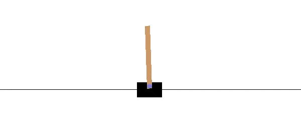
The Cartpole environment

A pole is attached by an un-actuated joint to a cart, which moves along a frictionless track (see the gif below). The system is controlled by applying a force between \(+10\) to \(-10\) to the cart. The pendulum starts upright, and the goal is to prevent it from falling over. A reward of \(+10\) is provided for every timestep that the pole remains upright. The episode ends when the pole is more than \(15\) degrees from vertical, or the cart moves more than \(2.4\) units from the center.

Current implementations of the Cartpole environment on well-known frameworks such as rllab compute consider three separate terms (or objectives) for the reward function: a constant reward, ucost and xcost.

1) \(\mathbf{10}\): this is the constant reward that is provided for every instant that the cart is upright.

2) \(\mathbf{\text{uCost} = -1e-5*(\text{action}^2)}\) : this is a penalty that takes the action into account. Higher the action, the more negative this objective. Ideally, we want to apply as little force on the cart as required to make it stand. With \(\text{action}=0\), there is no penalty.

3) \(\mathbf{\text{xCost} = -(1 - np.cos(\text{pole_angle}))}\) : this is a penalty that is based on how upright the cart is, the more vertical the better. Note that the angle here is measured from the pole’s upright position. Accordingly, for a perfectly vertical pole, \(\text{pole_angle}=0\) and \(\text{xCost} = 0\), while \(\text{xCost}=-1\) for a fallen pole that’s lying on the ground.

Along the lines of the single-objective or scalar reward function, the overall reward is simply taken to be the scalar sum of the three terms, i.e., \(10+\text{uCost}+\text{xCost}\).

The Pareto front

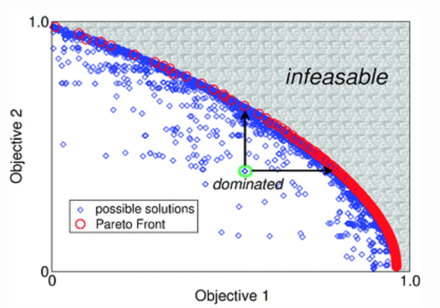
In the context of multi-objective optimization, there does not typically exist a feasible solution that minimizes (or maximizes) all objective functions simultaneously. Therefore, attention is paid to Pareto-optimal (or Pareto-dominant) solutions, which are defined to be solutions that cannot be improved in any of the objectives without degrading at least one of the other objectives.

Let us focus on a two-objective optimization problem for the purpose of understanding where we are looking to maximize both the objectives. Consider two distinct solutions on a two-dimensional space: \(S_1 = (x_1,y_1)\) and \(S_2 = (x_2,y_2)\). \(S_1\) is said to (pareto)-dominate solution \(S_2\) if

• \(x_1 > x_2\) and \(y_1 \geq y_2\)

OR

• \(x_1 \geq x_2\) and \(y_1 > y_2\)

In other words, \(S_1\) is better than (or equal to) \(S_2\) with respect to both the objectives, and hence dominates it.

The figure below (image courtesy [2]) provides a depiction of a Pareto front for the two-dimensional case. Notice that there are multiple solutions to this two-objective problem, that are marked blue. However, while many of these solutions are dominated by other solutions; it is only the red points that are non-dominated, and those form the Pareto front. Points under the Pareto front are feasible while those beyond the Pareto front are infeasible.

In the case of two continuous objectives, the Pareto front is a curve obviously consisting of potentially an infinite number of points. In practise the Pareto front is discretized and the points are tried to be located as evenly as possible on the front.

A methodology for considering the rewards separately

We now describe the \(\textbf{radial algorithm}\) introduced in [3] that presents a method to obtain the points on the Pareto front. We elucidate the concept for a two-dimensional scenario, specifically in the context of Policy Gradient algorithms.

Consider the two extreme steepest ascent directions (one for each objective) that maximize each objective and neglect the other objective. These directions are given by \(\theta_1=\nabla{_\theta} J_1(\theta)\) and \(\theta_2=\nabla{_\theta} J_2(\theta)\), where \(J_i=\mathbb{E}R_i\), and \(R_i\) is the reward along axis \(i\). Any direction in between \(\theta_1\) and \(\theta_2\) will simultaneously increase both the objectives. As a consequence, a sampling of directions amidst the two extreme directions corresponds to pointing at different locations on the Pareto frontier. Every direction intrinsically defines a preference ratio over the two objectives. We uniformly sample the ascent direction space via a splitting parameter \(\lambda\in\{0,1\}\) and use the ascent direction \(\theta_{\lambda}=\lambda\times\theta_1+(1-\lambda)\times\theta_2\).

Equivalently, we may set the overall reward to \(R=\lambda\times R_1 + (1-\lambda)\times R_2\) and perform policy optimization with this modified reward function. This is because

where \(R=\lambda\times R_1 + (1-\lambda)\times R_2\)

Each direction (chosen by a specific \(\lambda\)) provides an unique solution to our optimization problem. By determining the set of non-dominated solutions, the Pareto boundary can be well approximated.

The psuedo-code for the algorithm for a two-dimensional reward function is as follows:

• \(\{\lambda^{(i)}\}_{i=1}^p\) <– uniform sampling of \([0,1]\).

• \(\textbf{for}\) \(i=1,\ldots,p\) \(\textbf{do}\):

  • Initialize policy network parameters.

  • \(\textbf{for}\) iteration in \(1,\ldots,N\) \(\textbf{do}\):

    • Collect trajectories with features (state, action, reward:(\(R_1\),\(R_2\)), nextState).

    • Set net reward \(R=\lambda^{(i)}\times R_1+(1-\lambda^{(i)})\times R_2\).

    • Implement a policy optimization algorithm using reward function \(R\).

  • Record the optimal network parameters \(\theta_i\) for the splitting parameter \(\lambda^{(i)}\).

• Determine the set of Pareto-optimal points, i.e., the set of objective values that are not dominated by one another.

• The Patero front is obtained by piecewise-linearly connecting the set of Pareto-optimal points obtained. Each point on any of these lines is attainable by time sharing between the end points of that line.

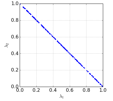
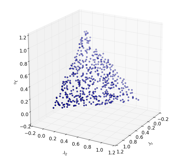
For a general case with \(n\) objectives, the Pareto front may be obtained by uniformly sampling from an \(n-1\)-dimensional hyperplane. Accordingly, we pick \(j=1,\ldots,p\) sets of the splitting parameters \((\lambda^{(j)}_1,\lambda^{(j)}_2,\ldots{},\lambda^{(j)}_n)\) subject to \(\sum_{j=1}^n\lambda^{(j)}_i = 1\), \(0 \leq\lambda^{(j)}_i\leq 1\), and the reward function \(R = \sum_{j=1}^n\lambda_j R_j\) is used.

• When \(n=2\), \(\lambda_1\) and \(\lambda_2\) are sampled from the line \(\lambda_1+\lambda_2=1\). The figure below shows \(200\) sampled points for the 2-D case.

• When \(n=3\), \(\lambda_1\), \(\lambda_2\) and \(\lambda_3\) are chosen from the equilateral triangle given by \(\lambda_1+\lambda_2+\lambda_3=1\) (see the figure below for a depiction of \(200\) randomly sampled points in this space).

Solutions to the Cartpole problem for the single and multiple objective cases

In the following, we solve the Cartpole problem using the vanilla policy gradient algorithm. We also consider three variants of the reward function. The following scenarios of objective functions are analyzed separately

• One-dimensional objective
  • We use the following simple scalar reward function: \(R=10+\text{xCost}+\text{uCost}\).
• Two-dimensional objective
  • We decompose the scalar reward used above into two objectives: \(R_1 = 10 + \text{xCost}\) and \(R_2=\text{uCost}\).
• Three-dimensional objective
  • Here, we treat all the reward components separately: \(R_1=10\), \(R_2=\text{xCost}\) and \(R_3=\text{uCost}\).

For the latter cases, we employ the radial algorithm to obtain the Pareto frontiers.

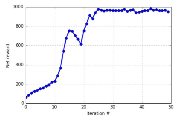
1) Scenario 1: The 1-D Reward Function

We ran the cartpole environment with the following hyperparameters:

N = 200 # number of trajectories per iteration
H = 100 # Horizon (each trajectory will have at most H time steps)
n_itr = 50 # number of iterations
discount = 0.99 # discounting factor
learning_rate = 0.01 # learning rate for the gradient update

The learning curve is plotted below for a single run (In practice, it is recommended to average over several runs). We see that the vanilla policy gradient algorithm learns quickly within about \(25\) iterations. With a horizon of \(100\) time steps, the net reward converges to around \(1000\) pertrajectory. This corresponds to a reward of \(10\) per time step, which is expected to be the optimum reward (when action\(\approx0\) and pole-angle\(\approx0\)).

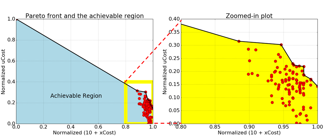
2) Scenario 2: The 2-D Reward Function

In the two objective case, the total reward can be decomposed as \(R_1=10+\text{xCost}\) and \(R_2=\text{uCost}\). We use the radial algorithm to solve the cartpole problem for the 2-D reward scenario and the Pareto front is depicted below. The figure on the left plots the achievable region and the figure on the right is a zoomed-in plot of the Pareto front. in this experiment, we considered \(p=100\) uniformly sampled values of \(\lambda_1\) and \(\lambda_2\).

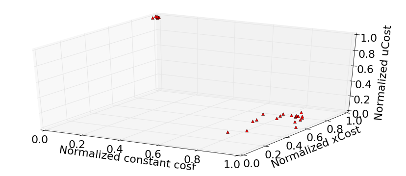
3) Scenario 3: The 3-D Reward Function Here, we extend the 2-D case by decomposing the total reward into \(R_1=10\), \(R_2=\text{xCost}\) and \(R_3=\text{uCost}\). The weighting factors for the rewards \((\lambda_1,\lambda_2,\lambda_3)\) are uniformly sampled from the equilateral triangle with vertices at \([0,0,1]\), \([0,1,0]\) and \([1,0,0]\). For the vanilla policy gradient, we use the reward function \(R=\lambda_1\times R_1 + \lambda_2\times R_2+(1-\lambda-1-\lambda_2)\times R_3\). See the figure below for a depiction of some Pareto-optimal solutions in the 3-D case.

Concluding Remarks

In this blog post, we have demonstrated how to handle reinforcement learning problems with multiple objectives by introducing the notion of a Pareto frontier. We also explain how to extend the mathematical concepts derived for the scalar reward case in the specific context of policy gradient algorihms to higher dimensions via the radial algorithm. A key point to note is with \(p\) splitting parameters, the time complexity grows \(p\)-fold, i.e., linearly with \(p\). More importantly, for an \(n\)-dimensional reward function, the number of sampling points \(p\) required to cover the sampling space grows exponentially with \(n\) (\(n-1\) to be precise). Thus, in comparison to an \(O(T)\) time complexity for the policy gradient algorithm using the scalar reward function, the policy gradient algorithm employing a \(n\)-dimensional reward function imbibes a time complexity of \(O(T^n)\)!

References

[1] J. Nocedal and S. J. Wright, Numerical Optimization

[2] J. Alander, A course on Evolutionary Computing

[3] S. Parisi et al., Policy gradient approaches for multi-objective sequential decision making IEEE International Joint Conference on Neural Networks (IJCNN), July 2014.